Question - Tune 3D Function
The student is given two superimposed surfaceplots, and a surface equation (z = f(x,y)) with a number of unkown parameters. One of the surfaceplots corresponds to the “correct” function, while the other lets the student “tune” the unkown parameters. The student needs to find the values of the parameters that makes the two surfaceplots coincide
Question description
If we wanted to randomize the goal function, the parameter values and/or the number of unkown parameters then getting data to and from jsxgraph with the usual {# … #}-notation and binding of sliders/points gets difficult. In this tutorial we will explore how we can deal with dynamic Input/output to jsxgraph.
We will also implement a clickable button that hides/shows an additional jsxgraph-figure and let control elevation/rotation of both figures from the control sliders on one of them.
Pedagogical Motivation
The goal of this excercise is for the student to examine what effect different parameters of a multivariable function has on the plot of its graph.
The move from 2D to 3D challenges the students intuition about functions and their algebraic components. By observing the effect dynamically changing some parameter of a function has on a graph while trying to fit it to a certain shape, we hope to build some intuition on the role of said parameter in a specific function.
Implementation
The version implemented here is supposed to be flexible with regards to which function and which and how many parameter the student is to examine.
The teacher should be able to choose any kind of function with a set of parameters to be examined by creating a function and a couple of lists in maxima. The only parts of the javascript code that could need editing is the parts that determines the size of the axes.
Student View
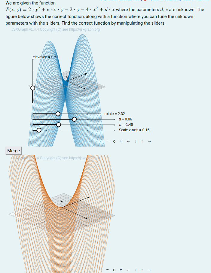
The student needs to manipulate the sliders corresponding to a parameter in the function such that the two surfaceplots coincide. Depending on the functions, this can initially be difficult when the plots are occupying the same figure. In that case the student can click a button that splits the graphs into to seperate figures, and merge them again for “fine- tuning”. When the graphs are split the rotation/elevation controls of the top figure controls the viewing angles of both plots. The student can also “scale” the z-axis to aid in a clear view of the plots.
Question Code
Question Variables
/*Non-randomized small example*/

func: a*x^2+b*x*y+c*y^2;
all_params: [a,b,c];
coef: [1,2,3];
params: [b];
param_sliders: [-4,0,4];

/*Randomized big example*/
/*
func: a*x^2+b*y^2+c*x*y+d*x+f*y+g;
all_params: [a,b,c,d,f,g];
coef: random_permutation(append([0,0],makelist(rand_with_prohib(-4,4,[0]),4)));
params: rand_selection(all_params,2);
param_sliders: [-4,0,4];
*/

/*x- and y- ranges */
xrang:[-7,7];
yrang:[-7,7];

/* Max error for tunable parameters */
maxError:0.2;

/*List of non-tunable parameters*/
non_params: sublist(all_params, lambda([x], not member(x, params)));

/*Stack-map, example: ["stack-map",
   ["a", 1], ["b", 2], ["pnames", ["a","b"]], ["sliders, [-4,0,4]]
]*/
params_json: append(["stack_map"],
   makelist([string(all_params[i]),coef[i]], i, length(all_params)),
   [["pnames", map(string,params)]], [["sliders", param_sliders]]
);

/*Parameter equation lists, example [a=1, b=2, c=3]*/
all_params_eq: makelist(all_params[i] = coef[i], i, length(all_params));
params_eq: sublist(all_params_eq, lambda ([x], member(lhs(x), params)));
non_params_eq: sublist(all_params_eq, lambda([x], member(lhs(x), non_params)));

/*Function evaluated with un-tunable parameters*/
fxy:ev(func,non_params_eq);

/*Function evaluated with all parameters given*/
fxy2:ev(func,all_params_eq);
In the question variables, the following part is expected to be changed by the teacher
func: a*x^2+b*y^2+c*x*y+d*x+f*y+g;
all_params: [a,b,c,d,f,g];
coef: random_permutation(append([0,0],makelist(rand_with_prohib(-4,4,[0]),4)));
params: rand_selection(all_params,2);
param_sliders: [-4,0,4];
xrang:[-7,7];
yrang:[-7,7];
maxError:0.2;
The variable func is the goal function, where the list all_params lists
the name of all “potentially unknown” parameters. The list coef holds all the
parameters values. In the example above, we have a 2. order polynomial with
6 parameters and they are given a random value between \([-4,4]\), excluding 0,
with two parameters guaranteed to be zero. The list params holds the names
of the unkown parameters, in the above example we draw two random parameters.
The last 4 lines above sets the ranges and starting values of the sliders, the x-, and y- domain and the tolerance of the students answer.
The rest of the maxima code should not need to be changed,
and does a couple of things. It creates som formatted parameter lists and two
functions. fxy is the function with only the known parameters evaluated,
fxy2 is the function with all parameters evaluated.
To get the data from maxima to jsxgraph, the easiest way usually is to use {#<CAS expression>#} syntax. This “pastes” the maxima result between # directly into the javascript-code. This would probably suffice in this case, but if the data is big/complex/dynamic it could be a good idea to use a stackmap in maxima that can be converted and parsed into a JSON object in the jsxgraph block.
A strackmap consists of a list that starts with the string “stackmap” followed by a variable number of sublists of length 2. The first element of the sublists is the “key” and the second element is the “value”.
params_json: append(["stack_map"],
   makelist([string(all_params[i]),coef[i]], i, length(all_params)),
   [["pnames", map(string,params)]], [["sliders", param_sliders]]
);
The above code creates the stackmap. It holds the the value of the parameters, the names of the parameters and the slider sizes. It could look something like this:
["stackmap",
    ["a",2],["b", 1],["c",-3],
    ["pnames", ["a","b"]],
    ["sliders", [-4,0,4]]
]
This can be converted and parsed into a JSON object, which we use to access the data from maxima:
 var stack_input = JSON.parse({#stackjson_stringify(params_json)#});
 var paramater_names = stack_input["pnames"];
 var param_a_value = stack_input["a"];
Question Text
Usually would want one hidden input box bound to each slider that is part of the students answer. In this case we might not know the name of, or more importantly, the number of sliders. In such cases we can manually “bind” all the relevant data form jsxgraph to a single answer variable/input box:
<p style="display:none">[[input:ans]] [[validation:ans]]</p>
The question text proper is straight forward.
We are given the function \(F(x,y) = {@fxy@}\) where
the parameters \({@simplode(params,",")@}\) are unknown.
The figure below shows the correct function, along with a function
where you can tune the unknown parameters with the sliders.
Find the correct function by manipulating the sliders.
The critical part is the javascript code, in [[jsxgraph]] tags.
Coding the Plot
[[jsxgraph input-ref-ans="ansRef"]]
(function () {

   //Get divid for bottom jsxgraph figure by
   //incrementing number in divid of top figure
   //
   //Regex that matches number between 1-99
   var regexMatchNumber = /([1-9][0-9]|[1-9])/g;
   var nextDivNum = Number(divid.match(regexMatchNumber))+1;//Match+increment
   var divid2 = divid.replace(regexMatchNumber, nextDivNum);//Replace new number

   //Reference to the bottm jsxgraph figure
   var jsxgraph2 = document.getElementById(divid2);
   jsxgraph2.style.display="none";//Hide second figure by default


   //{#stackjson_stringify(params_json)#} inserts JSON string from maxima
   //JSON.parse() returns a JSON object of the data from maxima
   var stack_input = JSON.parse({#stackjson_stringify(params_json)#});
   var ans = document.getElementById(ansRef);//Reference to answer field
   ans.value= JSON.stringify(stack_input); //Write JSON object to ans as string

   // Create the board
   var board = JXG.JSXGraph.initBoard(divid, {
      boundingbox: [-11 ,11, 11, -11],
      keepaspectratio: false,
      axis: false
   });


   //Create the 3D view
   var box = [-2, 2];
   var boxx = {#xrang#};
   var boxy = {#yrang#};
   var view = board.create('view3d', [[-6, -3], [8, 8], [boxx, boxy, box]], {
      xPlaneRear: {visible: false},
      yPlaneRear: {visible: false},
   });

   //Array of strings containing the names of the tunable parameters
   //Example: ["a", "c",...]
   var pnames = stack_input["pnames"];

   //Start, initial and stop value of sliders
   var slider_size = stack_input["sliders"];

   var sliders = []; //Array holding a reference to sliders

   //For several sliders, we need to shift the y-position so they don't overlap
   var slider_shift = 0

   // Iterate over the the names of the tunable parameters
   for (var i=0; i<pnames.length; i++){

      //Set the initial tunable parameter value to startvalue of sliders
      stack_input[pnames[i]] = slider_size[1];
      //Write new parameter values to answer field
      ans.value = JSON.stringify(stack_input);


      //Create and push new slider to list of sliders
      sliders.push(board.create('slider',
         [[-7, -6-slider_shift], [5, -6-slider_shift], slider_size],
         { name: pnames[i] }//New slider has same name as the parameter
      ));
      slider_shift++; //Shift y-position for next slider

      board.update();
   }

   //Create the scaleing slider for the function plot
   var scale_slider = board.create('slider',
      [[-7,-6-slider_shift],[5,-6-slider_shift], [0,1,2]],
      {name: "Scale z-axis"}
   );

   // JessieCode parsing of maxima function "fxy" - tunable
   var ff = board.jc.snippet('{#fxy#}', true, 'x,y', true);

   // The function f calls the tunable function ff, andj scales it
   // by mulitplying with z-axis slider
   var f = (x,y) => scale_slider.Value()*ff(x,y);

   //Create the 3D tunable surface
   view.create('functiongraph3d', [f, boxx, boxy], {
      strokeColor: JXG.palette.blue,
      stepsU: 50, stepsV: 50, strokeWidth: 0.5
   });


   //JessieCode parsing of maxima function "fxy2"- non-tunable
   var gg = board.jc.snippet('{#fxy2#}', true, 'x,y', true);
   // g(x,y) calls gg(x,y) but scales it with the slider
   var g = (x,y) => scale_slider.Value()*gg(x,y);

   //Create the 3D non-tunable function
   var func_g = view.create('functiongraph3d', [g, boxx, boxy], {
      strokeColor: JXG.palette.red,
      stepsU: 50, stepsV: 50, strokeWidth: 0.5
   });

   //Create a second board for the jsxgraph figure below (divid2)
   var board2 = JXG.JSXGraph.initBoard(divid2, {
      boundingbox: [-8, 8, 8, -8],
      keepaspectratio: false,
      axis: false
   });

   //Add board2 as a child to board - the bottom figure updates automatically
   //when the student manipulates the top figure
   board.addChild(board2);

   //Create 3D view for botoom figure
   var view2 = board2.create('view3d',
      [[-6, -3], [8, 8], [boxx, boxy, box]], {
      xPlaneRear: {visible: false},
      yPlaneRear: {visible: false},
   });

   //Create 3D non-tunable surface in bottom figure
   view2.create('functiongraph3d', [g, boxx, boxy], {
      strokeColor: JXG.palette.red,
      stepsU: 50, stepsV: 50, strokeWidth: 0.5
   });
   board2.update();

   //We want to control rotation and elevation of bottom figure
   //with the controls in the top figure
   //Hide the controls in bottom figure
   view2.D3.az_slide.hide();
   view2.D3.el_slide.hide();
   //Set the rotation and elevation of bottom figure to
   //that of the first figure
   view2.D3.az_slide = view.D3.az_slide;
   view2.D3.el_slide = view.D3.el_slide;

   //Rename elevation and rotation control sliders
   view.D3.el_slide.name = "elevation";
   view.D3.az_slide.name="rotate";
   board.update();

   // Set event listener for button that allows student
   // to split the tunable and non-tunable surfaces into different figures
   //
   // Get reference to clickable button
   var button = document.getElementById('split-button');
   //Add the function to be called when the button is clicked
   button.addEventListener('click', function() {

      // If value=0 we hide the goal-plot and show the bottom figure
      if (button.value == "0"){
         func_g.hide();                     //Hide target function
         button.value = "1";                //Toggle button value
         button.textContent = "Merge";      //Toggle button text
         jsxgraph2.style.display = "block"; //Show bottom figure
      }
      else { //If value != 0 we show the goal-plot and hide the bottom figure
         func_g.show();                    //Show target function
         button.value="0";                 //Toggle button value
         button.textContent = "Split";     //Toggle button text
         jsxgraph2.style.display = "none"; //Hide bottom figure
      }
   });

   //Add a function that updates the answer variable going out to STACK
   //everytime the board changes
   board.on('update', function(){
      for (let i=0; i<sliders.length; i++) //Iterate over tunable sliders
      {
         var ans_name = sliders[i].getAttribute("name"); //Get name of slider
         stack_input[ans_name] = sliders[i].Value();  //Update value of parameter
      }
      //Write JSON object with updated parameter values to stack answer field
      ans.value=JSON.stringify(stack_input);
   });

})();
[[/jsxgraph]]
The jsxgraph block starts with
[[jsxgraph input-ref-ans="ansRef"]]
In the opening jsxgraph block we specify that we want a reference to the STACK answerfield “ans” stored in a variable “ansRef”
Then we get the ID of the bottom jsxgraph figure. We want the students
to be able to toggle between showing both graphs in a single figure
or seperate figures by clicking a button.
The code for both plots is contained in the first jsxgraph block.
The ID for the jsxgraphblock is contained in divid and has value
“stack-jsxgraph-X”, where X is a number controlled by stack, depending on
how many jsxgraph figures is on the quiz page. We can get the ID of the
bottom graph by incrementing X for the first graph, which we do with regex:
   var regexMatchNumber = /([1-9][0-9]|[1-9])/g;
   var nextDivNum = Number(divid.match(regexMatchNumber))+1;//Match+increment
   var divid2 = divid.replace(regexMatchNumber, nextDivNum);//Replace new number
We use divid2 to get a reference to the bottom figure, in order
to hide/show it.
   var jsxgraph2 = document.getElementById(divid2);
   jsxgraph2.style.display="none";//Hide second figure by default
The two boards an 3Dviews can now be created in their respective figures
   var board = JXG.JSXGraph.initBoard(divid, {...
   var board2 = JXG.JSXGraph.initBoard(divid2, { ...
   var view = board.create('view3d', ....
   var view2 = board2.create('view3d', ....
Next we nee to get our data from maxima.
The maximafunction stackjson_stringify(params_json) encodes the stackmap
into a JSON string, which we can parse into a JSON object with JSON.parse()
   var stack_input = JSON.parse({#stackjson_stringify(params_json)#});
   var ans = document.getElementById(ansRef);//Reference to answer field
   ans.value= JSON.stringify(stack_input); //Write JSON object to ans as string
We also get the answerfield element by using our supplied “ansRef” reference, and store our stack_input object as string in the answerfield with JSON.stringify. The goal is to hand the position of the sliders back to stack, by updating the stack_input object with the current slider values and write the entire object back to the answerfield.
From the stack_input object we can get the slider sizes and the parameter names:
   var pnames = stack_input["pnames"];
   var slider_size = stack_input["sliders"];
We can now create the sliders for the tunable parameters:
   var sliders = []; //Array holding a reference to sliders

   //For several sliders, we need to shift the y-position so they don't overlap
   var slider_shift = 0

   // Iterate over the the names of the tunable parameters
   for (var i=0; i<pnames.length; i++){

      //Set the initial tunable parameter value to startvalue of sliders
      stack_input[pnames[i]] = slider_size[1];
      //Write new parameter values to answer field
      ans.value = JSON.stringify(stack_input);


      //Create and push new slider to list of sliders
      sliders.push(board.create('slider',
         [[-7, -6-slider_shift], [5, -6-slider_shift], slider_size],
         { name: pnames[i] }//New slider has same name as the parameter
      ));
      slider_shift++; //Shift y-position for next slider

      board.update();
   }
The sliders are given the same name as the tunable parameters, which means they will affect the functionplot. Also note that we set the parameter values in stack_input to the initial value of the corresponding slider and write it to the answerfield. Otherwise the answerfield would initially contain the correct values.
Next we parse the functionstrings fxy and fxy2 from maxima with with <board>.jc.snippet(), create the scaled function to be plotted and plot the functions in the same manner as in previous tutorials.
The point of having the option to view the plots in seperate figures, is that it can be messy and difficult to match the plots in the same figure initially. We also want the same rotation and elevation angles in the two plots at all times, which we can accomplish by hiding the el. az. controls in the bottom figure and set the controls in the first figure to also control the bottom figure:
   view2.D3.az_slide.hide();
   view2.D3.el_slide.hide();

   view2.D3.az_slide = view.D3.az_slide;
   view2.D3.el_slide = view.D3.el_slide;

   //Rename elevation and rotation control sliders
   view.D3.el_slide.name = "elevation";
   view.D3.az_slide.name="rotate";
The button itself is added in html between the two jsxgraph-blocks:
<button type="button" value="0" id="split-button"> Split </button>
Its logic is added made as follows:
   var button = document.getElementById('split-button');
   //Add the function to be called when the button is clicked
   button.addEventListener('click', function() {

      // If value=0 we hide the goal-plot and show the bottom figure
      if (button.value == "0"){
         func_g.hide();                     //Hide target function
         button.value = "1";                //Toggle button value
         button.textContent = "Merge";      //Toggle button text
         jsxgraph2.style.display = "block"; //Show bottom figure
      }
      else { //If value != 0 we show the goal-plot and hide the bottom figure
         func_g.show();                    //Show target function
         button.value="0";                 //Toggle button value
         button.textContent = "Split";     //Toggle button text
         jsxgraph2.style.display = "none"; //Hide bottom figure
      }
   });
The final piece of the puzzle is to make sure to write an updated JSON object as a string to the answerfield everytime the student manipulates the figure:
   board.on('update', function(){
      for (let i=0; i<sliders.length; i++) //Iterate over tunable sliders
      {
         var ans_name = sliders[i].getAttribute("name"); //Get name of slider
         stack_input[ans_name] = sliders[i].Value();  //Update value of parameter
      }
      //Write JSON object with updated parameter values to stack answer field
      ans.value=JSON.stringify(stack_input);
   });
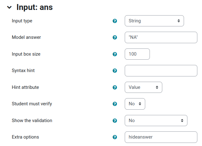
Input:ans
 |
|---|
| Input setting for answervariable “ans” |
For the answer variable ans, we set the input type to “String”. The model answer is not really applicable since the variable stores several things, and we put “NA” here. We also set the option “hideanswer” in the extra options box, to stop the student getting freedback regarding the answer variable
Partial Response Tree
Feedback variables
The feedback variables does two main things: It parses the JSON-string
contained in the answer variables and collect the student’s answer,
and it checks if the tunable parameters given by the student
are within the set tolerance maxErrorof the correct values.
/*Parse json-string from jsxgraph*/
tmp:stackjson_parse(ans);

/*Student answer example [[a,4], [b,6], ... ]*/
sanswer:map(lambda([x], [x,stackmap_get(tmp, string(x))]), params);

/*Teacher answer */
tanswer:map(lambda([x], [lhs(x), rhs(x)]), params_eq);

/*Find parameterval for par in tanswer*/
findParameterVal(par):=
   (sublist(tanswer, lambda([x], is(equal(x[1],par)))))[1][2];

/*List of errors in the parameters, example [[a,0], [b,0.35], [c,0]] */
errors:makelist( [sanswer[i][1],
   abs(sanswer[i][2]-findParameterVal(sanswer[i][1]))],
   i,1,length(sanswer));

/*List of correct parameters (error<maxError) */
correct:sublist(errors, lambda([x], x[2]<maxError));
/*Formatted list of correct parameters */
correct_list:sublist(params_eq,
   lambda([x], member(lhs(x), map(first, correct))));

/*List of incorrect parameters*/
incorrect:sublist(errors, lambda([x], x[2]>=maxError));

/*Number of correct answers*/
n_stud:length(correct);
n_ans:length(tanswer);
To get a hold of the variables in the JSON string,
we use tmp:stackjson_parse(ans).
This parses the JSON string from jsxgraph and returns a stackmap.
We can then use the function stackmap_get(<stackmap>, <key>) to lookup
the value of a key in the stackmap.
We look up the values for all tunable parameters and store them in a list
sanswer = [[<parameter>, <value>], ...] here:
sanswer:map(lambda([x], [x,stackmap_get(tmp, string(x))]), params);
The list tanswer is of the same form, and contains the correct
parameter names/values.
Next we calculate a list of the student’s error and filter out the parameters whose error is above the tolerance.
findParameterVal(par):=
   (sublist(tanswer, lambda([x], is(equal(x[1],par)))))[1][2];

errors:makelist( [sanswer[i][1],
   abs(sanswer[i][2]-findParameterVal(sanswer[i][1]))],
   i,1,length(sanswer));

correct:sublist(errors, lambda([x], x[2]<maxError));
correct_list:sublist(params_eq,
   lambda([x], member(lhs(x), map(first, correct))));
We have to use the function findParameterVal(par) to look up the correct
parameter value in tanswer as the parameternames not necessarily are
in the same order after we in the question variables
form chose 2 random parameters.
The variables n_stud and n_ans hold the number of correctly tuned parameters,
and the total number of parameters, respectively
Response Tree Nodes
The response tree is quite straightforward - It compares the number of correct
parameters from the student n_stud with the total number of tunable parameters
n_ans. If they are equal, the student gets full marks. If the student gets
at least 1 parameter right they get half marks, and otherwise no marks.