Question. Find a function with given properties
Ask the user to an algebraic expression defining a function in two variables with certain properties. Visualise the function as a surface plot, to help the student to validate the properties visually.
One example would be function where all the partial derivatives in a given point $(x,y)$ are (say) positive.
 |
|---|
| First impression of the question |
Question description
The question is simple, but the tutorial effectively illustrates how the algebraic answer in STACK can be linked to variables in JSXGraph and its visualisation.
Pedagogical Motivation
This exercise is an early training exercise when the student starts studying functions of two variables in calculus.
The visualisation trains the student in seeing the relationship between the algebraic and the graphical representation when solving problems.
The particular question aims to develop the intuitive understanding of the partial derivative.
Implementation
The version implemented here is quite flexible, including variants where each partial derivative may be required to be negative, positive, or zero. Thus the question will make the following calculation.
- Draw the sign of $f_x$ uniformly at random from ±1 and 0.
- Draw the sign of $f_y$ uniformly at random from ±1 and 0.
- Draw a random point $(x_0,y_0)$ such that $x,y\in{\pm1,\pm2,\ldots,\pm5}$, where the partial derivatives are restricted.
Student View
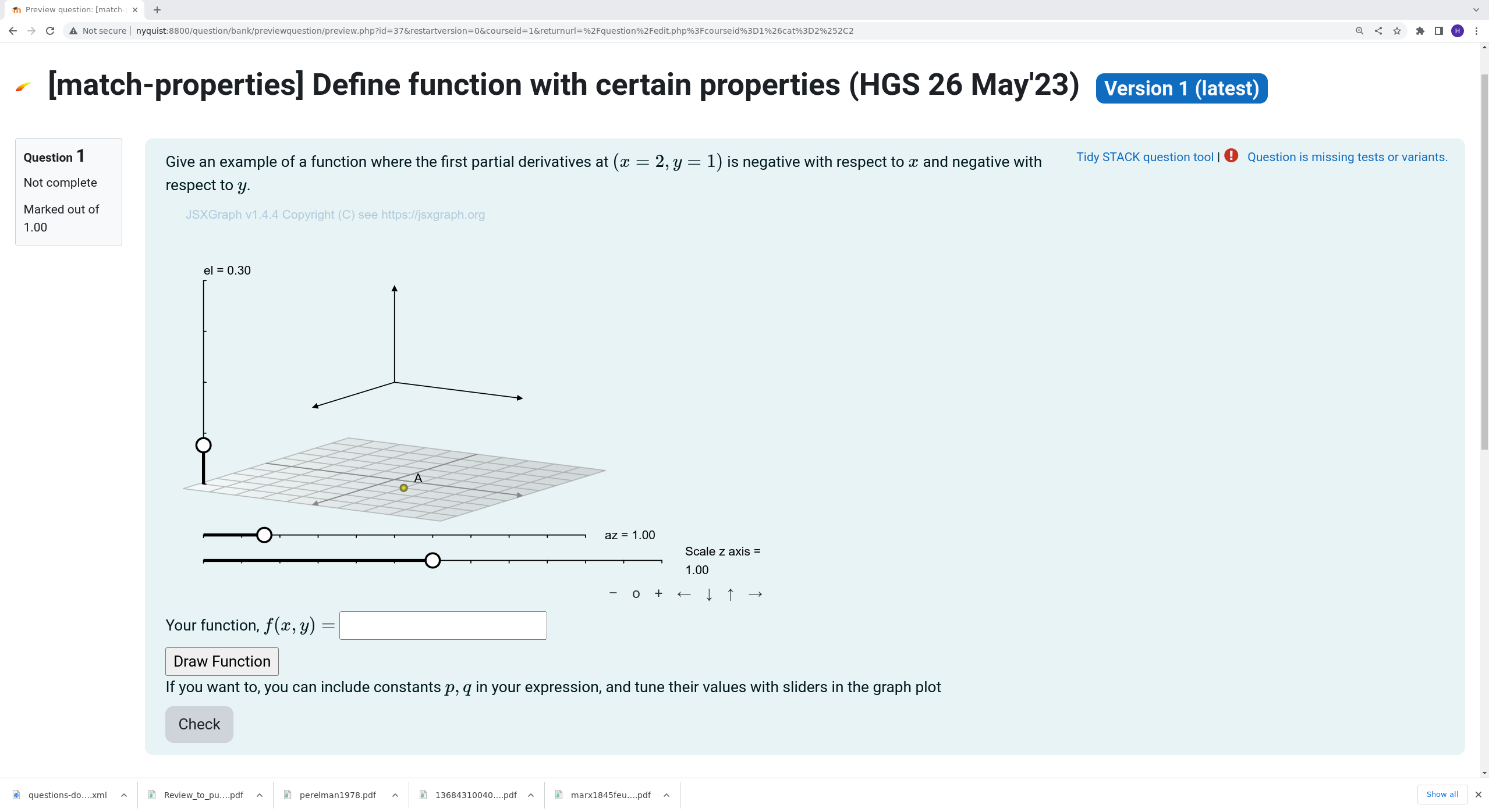
The question as implemented below includes several graphical features to visualise the problem and solution to the student.
 |
|---|
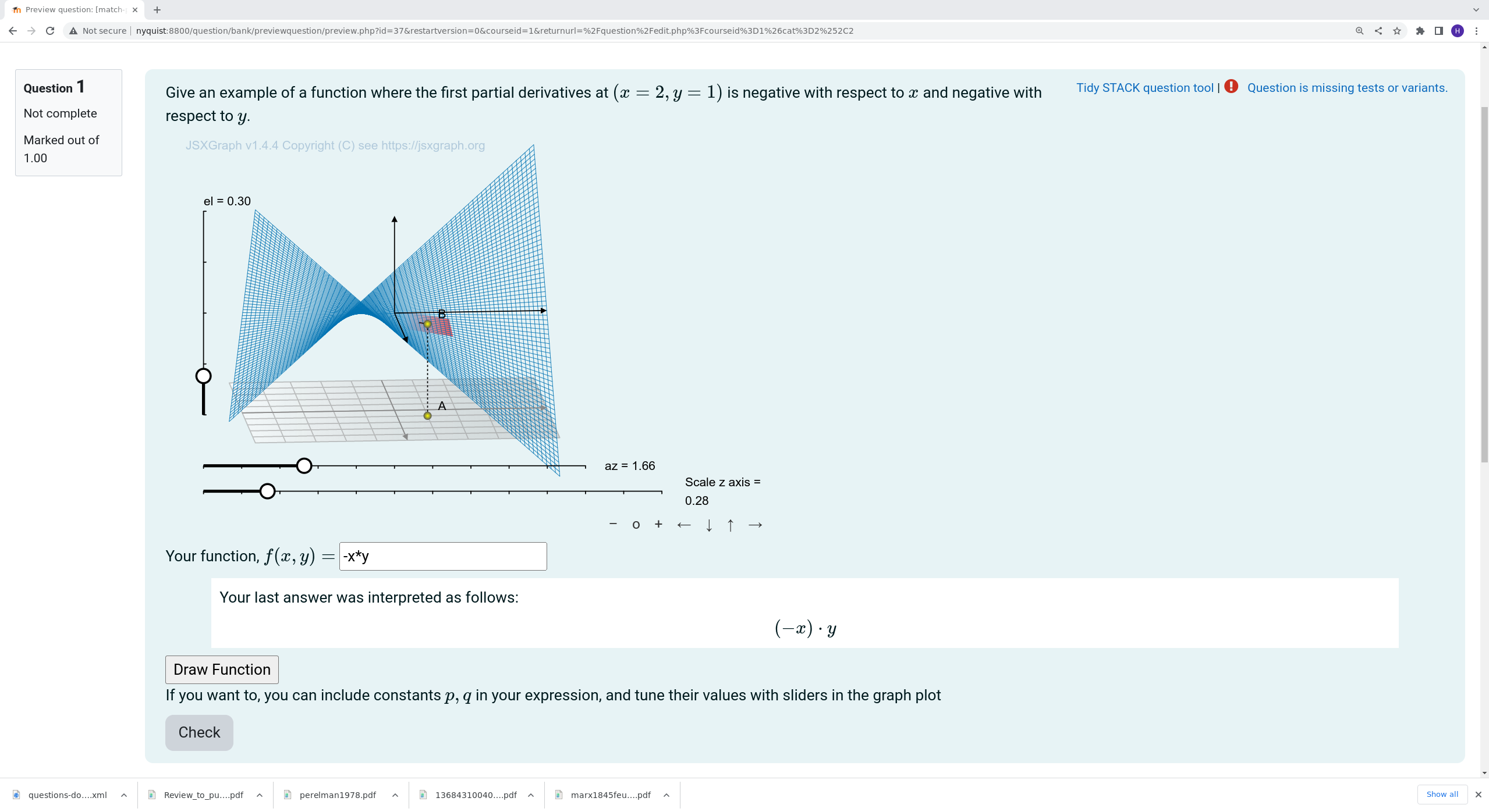
| When the student types in the function and clicks the Draw button |
The student has to enter an algebraic expression in $(x,y)$. They may parameterise the expression with $(p,q)$, in which case sliders appear, letting the smoothly and interactively adjust the parameters in the plot.
In addition to visualising the algebraic expression in $x$ and $y$, we also visualise the tangent plane in the reference point. This reference point can be moved by dragging.
Unfortunately, we cannot rotate and pan the view using mouse actions directly on the 3D plot. Instead the sliders have to be used, but at least the student can study the function from any angle.
We have not found a way to draw the function automatically. Hence, the student has to click the `Draw Function’ button to see the plot.
Question Code
Question Variables
The question variables comprise the point $(x_0,y_0)$, the signs of the partial derivatives, and a model answer, as follows:
x0: rand_with_prohib(-5,5,[0]);
y0: rand_with_prohib(-5,5,[0]);

xsign: rand(3)-1;
ysign: rand(3)-1;

modelanswer: xsign*a*x^2 + ysign*b*y^2 ;
Question Text
The question text is nasty, because it has to include all the javascript code to manage the plot.
The first section is the main text of the question
<p>
  Give an example of a function where the first partial derivatives at
    \((x={@x0@},y={@y0@})\) is
     {@if xsign > 0 then "positive"
      else if xsign < 0 then "negative"
      else "zero"@}
     with respect to \(x\) and
     {@if ysign > 0 then "positive"
      else if ysign < 0 then "negative"
      else "zero"@}
     with respect to \(y\).
</p>
This is not quite ideal. In the case where the partial derivativs have the same sign, it would be better to merge the two clauses into one and write e.g. «both partial derivatives are positive».
In addition to the student answer ans1, we need three hidden answers.
The first two, p1 and p2 are the parameters $p$ and $q$ which the
student can use in their answer. The third onw is a state variable which
would be needed if the question is extended to a multi-part question, so
that the plot can be restored after a page change.
<p style="display:none">[[input:p1]][[validation:p1]]</p>
<p style="display:none">[[input:p2]][[validation:p2]]</p>
<p style="display:none">[[input:stateStore]][[validation:stateStore]]</p>
The javascript code is discussed below. After the plot, we have to code to receive and validate the student answer.
<p>Your function, \(f(x,y) =\) [[input:ans1]][[validation:ans1]] </p>
<input type="button" value="Draw Function" id="draw_button">
<p>If you want to, you can include constants \(p, q\) in your expression,
   and tune their values with sliders in the graph plot </p>
Coding the Plot
The javascript code is enclosed in special STACK tags, which not only indicates javascript but also loads the required libraries. The opening tag has to specify the size of the plot and all the student answer fields used, including the hidden once.
[[jsxgraph height='850px' width='850px' input-ref-p1="pRef" input-ref-p2="qRef" input-ref-ans1="ans1Ref" input-ref-stateStore="stateRef"]]
[[/jsxgraph]]
The following javascript code belongs inside the jsxgraph tags.
First we set up the board.
   // This is the basic code to create 3D co-ordinate system and view
   var board = JXG.JSXGraph.initBoard(divid, {
      boundingbox: [-8, 8, 8, -8],
      keepaspectratio: false,
      axis: false
   });
   var box = [-5, 5];
   var view = board.create('view3d',
      [
         [-6, -3], [8, 8],
         [box, box, box]
      ],
      {
         xPlaneRear: {visible: false},
         yPlaneRear: {visible: false},
      });

   // Define a sliders to scale the z axis
   var scale_slider = board.create('slider', [[-7,-6],[5,-6],[0,1,2]],
          {name: "Scale z axis"});
Sliders to rotate the view are included in the default board. We add an extra slider to scale the $z$ axis in the last statement above.
We are going to visualise the tangent plane in a chosen point. We visualise this point and make it draggable in the $xy$ plane as follows.
   var p_bottom, p_graph, dashline;
   p_bottom = view.create('point3d', [1,1,-5]);
We need to make sliders for $p$ and $q$ and link them to the hidden answer fields. This is done as follows.
   // Initialise the hidden answer variables to avoid errors:
   var pref = document.getElementById(pRef);
   var qref = document.getElementById(qRef);
   pref.value = 1 ;
   qref.value = 1 ;

   var slider_p = board.create('slider', [[-7,-6.5],[5,-6.5],[-1,1,1]], {name: "p"});
   var slider_q = board.create('slider', [[-7,-7],[5,-7],[-1,1,1]], {name: "q"});
   // The p and q sliders are hidden until needed
   slider_q.hide();
   slider_p.hide();

   // We bind the parameters slides to STACK's answer variables
   // This let's Maxima use the values when grading
   stack_jxg.bind_slider(pRef,slider_p);
   stack_jxg.bind_slider(qRef,slider_q);
Note the last two lines in particular. This is shows the STACK binding to link a javascript variable to a STACK answer field.
Now comes the big step, of visualising the student answer.
We create a button with an event listener, and a function called
by the listener to draw the function.
Note that we need global variables to hold plot elements so that
subsequent calls to drawFunction() can remove old material.
   // Create the button and its listener
   let btn = document.getElementById("draw_button");
   btn.addEventListener("click", drawFunction);

   // The following variables hold board elements.
   // They are global so that drawFunction() can remove elements
   // from previous calls.
   var dFx, dFy, tangplane, tangx, tangy, scale_x, scale_y, F, funcExpr, fGraph;

   // drawFunction() is called from the button
   function drawFunction() {

      // We get the function expression supplied by student
      var ans1 = document.getElementById(ans1Ref);
      funcExpr = ans1.value;

      // Show $p$ and $q$ sliders only when needed
      if (funcExpr.includes("p")) {
         slider_p.show();
      } else {
         slider_p.hide();
      }
      if (funcExpr.includes("q")){
         slider_q.show();
      } else {
         slider_q.hide();
      }

      // Remove any previous graphs and planes
      board.removeObject(fGraph,false);
      board.removeObject(p_graph,false);
      board.removeObject(dashline,false);
      board.removeObject(tangplane,false);
      board.removeObject(tangx,false);
      board.removeObject(tangy,false);

      // We use a first order central difference to get numerical
      // approximations for Fx and Fy
      var h = 0.01 //Stepsize for finite difference
      var FF = board.jc.snippet(funcExpr, true, 'x,y', true);
                 // JessieCode parsing of function
      F = (x,y) => scale_slider.Value()*FF(x,y);
                 // Multiply function value with the scale_slider to scale it

      // Finite difference approximation of partial derivatives at the x-, y-
      // coordinates given by the draggable point on the bottom
      dFx = function () {
         var x = p_bottom.D3.X();
         var y = p_bottom.D3.Y();
         return (F(x+h,y)-F(x-h,y))/(2*h);
      }
      dFy = function () {
         var x = p_bottom.D3.X();
         var y = p_bottom.D3.Y();
         return (F(x,y+h)-F(x,y-h))/(2*h);
      }

      // Functions that gives the factor that normalizes the tangent plane
      scale_x = ()=> 1.0/Math.sqrt(1+Math.pow(dFx(),2));
      scale_y = ()=> 1.0/Math.sqrt(1+Math.pow(dFy(),2));

      // Draw the point on the graph that corresponds to the bottom point
      p_graph = view.create('point3d', [()=>p_bottom.D3.X(), ()=>p_bottom.D3.Y(),
                                         ()=>F(p_bottom.D3.X(), p_bottom.D3.Y())]);
      //Draw a dashed line between graph point and bottom point
      dashline = view.create('line3d', [p_bottom, p_graph], {dash: 1});

      // Draw the "unit" tangent plane (Area 2) - [point, [direction1], [direction2], [length1], [length2]
      // The directions are unit vectors from div(F) - the gives a factor of how much of the directions the plane spans
      tangplane = view.create('plane3d', [p_graph,
         [scale_x,0,()=>scale_x()*dFx()],
         [0,scale_y,()=>scale_y()*dFy()],
         [-0.8,0.8],[-0.8,0.8]],
         {fillOpacity: 0.8, fillColor: 'red'}
      );

      // Gradient lines
      tangx = view.create('line3d', [p_graph, [1,0,dFx],[0,dFx]]);
      tangy = view.create('line3d', [p_graph, [0,1,dFy],[0,dFy]]);

      // Plot the graph
      fGraph = view.create('functiongraph3d', [ F, box, box, ],
                { strokeWidth: 0.5, stepsU: 70, stepsV: 70 });
      board.update();

   }; // drawFunction
The last step is state management. This may not be needed in this question, but it would be needed when making multi-page questions.
   // Get reference to the hidden answer holding the board state
   var state = document.getElementById(stateRef);

   // If the state has been set, we need to restore the state from
   // previous work by the student.
   if (state.value && state.value != "") {
      //Parse the string-representation of the state
      var newState = JSON.parse(state.value);

      //Update the different, sliders to previous state
      scale_slider.setValue(newState["scale_slider"]);
      slider_p.setValue(newState["slider_p"]);
      slider_q.setValue(newState["slider_q"]);
      //elevation and rotation sliders
      view.D3.el_slide.setValue(newState["el_slider"]);
      view.D3.az_slide.setValue(newState["az_slider"]);
      //Bottom control point
      p_bottom.D3.coords = newState["p_bottom"];

      board.update();

      //Read function expression and draw everything at the end
      funcExpr = newState["funcExpr"];
      drawFunction();

   }

   // When the board updates, we need to update the state variable
   board.on('update', function() {
      //JSON object to contain the state of the board
      var newState = {};
      //Add all the entries we want to "save"
      newState.scale_slider = scale_slider.Value();
      newState.slider_p = slider_p.Value();
      newState.slider_q = slider_q.Value();
      newState.el_slider = view.D3.el_slide.Value();
      newState.az_slider = view.D3.az_slide.Value();
      newState.funcExpr = funcExpr;
      newState.p_bottom = p_bottom.D3.coords;
      //Store the state in the stateStore answer field as a string
      state.value = JSON.stringify(newState);
   });
Model Answers
The model answers have to be filled in, for ans1, p1, p2, and stateStore.
Mostly, the defaults are fine; all the answers are algebraic input, but a few
changes are necessary.
For ans1 we defined the modelanswer in maxima (above). This has to be entered
as the Model answer.
For the other three answers, there is no meaningful model answer, so any valid value would
do; say NA for stateStore and 1 for p1 and p2.
Importantly, these answers should be hidden from the student, which requires the keyword
hideanswer to be entered under Extra options (last in the Input: … section).
Partial Response Tree
We define only one PRT, with two nodes, one to check each of the partial derivatives. The student gets ½ point for each satisfied criterion. A perfect answer thus gets one point, and partially correct answers are possible.
Feedback variables
The following variables have to be defined, calculating the partial
derivatives and finding their signs in the reference point.
We also the word array to translate a numeric sign into a word to use
in the feecback text.
fx: diff(ans1,x);
fy: diff(ans1,y);
evfx: ev(fx,x=x0,y=y0);
evfy: ev(fy,x=x0,y=y0);
signfx: signum(evfx) ;
signfy: signum(evfy) ;
word : [ "negative", "zero", "positive" ] ;
The nodes
The two nodes should check signfx (resp. signfy) as SAns against xsign
(resp. ysign) as TAns.
Using the default algebraic equivalence (AlgEquiv) as Answer test is
ok, but other tests work too.
The Score should be 0.5 for true and 0 for false, and importantly, we have to change
the Mod to + so that the scores from each node are added together.
Each node should have a feedback text. When the $x$ derivative is correct, we can use.
<p>Your function, \(f(x,y) = {@ans1@}\) has partial derivative
\(f_x = {@fx@}\) which  evaluates to
\(f_x({@x0@},{@y0@}) = {@evfx@}\)
which is {@word[2+signfy]@} as required.
</p>
When the derivative is wrong, we may instead use,
<p>Your function, \(f(x,y) = {@ans1@}\) has partial derivative
\(f_x = {@fx@}\) which  evaluates to
\(f_x({@x0@},{@y0@}) = {@evfx@}\)
which is {@word[2+signfy]@},
but it should have been {@word[2+xsign]@}.
</p>
It should be trivial to edit these to make corresponding texts for the other node.