Point with negative-definite Hessian
Aim of task
- Student understands how the Hessian matrix is used in Taylor approximation to locally approximate functions (Communicating in, with, and about mathematics)
- Student understands, how local approximation and value of Hessian matrix are connected graphically (Representing mathematical entities)
- Using a visualization of Taylor-approximation student can derive qualitative statements about Hessian matrix at a given point (Making use of aids and tools)
 |
|---|
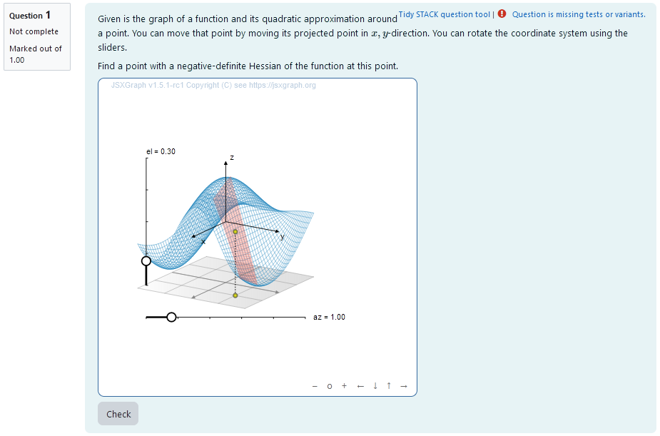
| First impression of the question |
Question description
A 2D function is plotted and its Taylor approximation of second order is given at a moveable point $x= (x_1,x_2)$. Since the Taylor approximation is given as \(f_2 (t) = f(x_0) + \nabla f(x_0) \cdot (x-x_0) + \frac{1}{2} (x-x_0)^\text{T} H_f(x-x_0)\) the character of the Taylor approximation gives information about the hessian of the function.
The student needs to find a point $(x,y)$, where the Hessian of the function is negative-definite.
Student perspective
When the point is moved in $x-y$-direction, the height of a corresponding point with the same $x,y$-coordinates moves according to the 2D-function. At this point, the local quadratical taylor approximation is calculated and plotted in a range big enough to estimate the infinite development.
The student moves the plane to a point with an approximation that fulfils the requirements. The coordinates of the points are interpreted as answers.
|  |
|:–:|
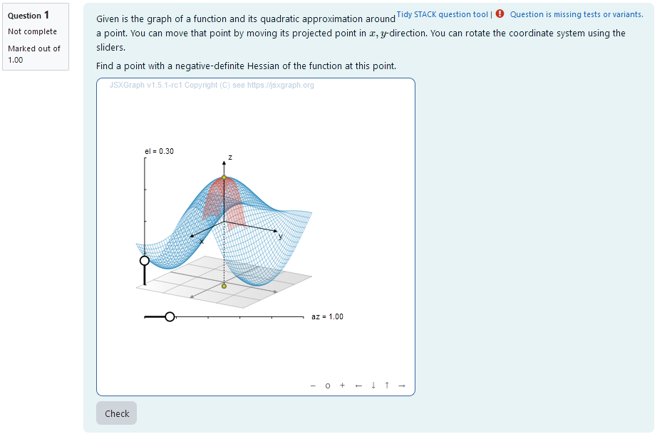
| When the student solves the problem |
|
|:–:|
| When the student solves the problem |
Feedback example
 |
|---|
| Feedback on answer above |
Teacher perspective
The teacher is able to give a list of possible values for parameters of the function. In order to do this, they simply need to modify the entries in the lists specified e.g. change a1: rand([2,4,6,8,10])/5 to a1:rand([2,3,4,5,6,7,8])/5.
Additionally, they can change the possible values for the $x$ and $y$ off-sets x0 and y0. This offset is used to counteract the fact, that $(0,0)$ is a common stationary point.
Furthermore the teacher is able to change the function entirely to a function that fits his needs. They can change the function defined by F: -a1 * cos(%pi*a2 * (x-x0))* cos(%pi* a3 * (y-y0)); to a function they desire. However, it might be necessary to define additional parameters analogous to the ones defined before.
Lastly, the reference solution RefSolx andRefSoly for an exemplatory stationary point must be adjusted to the function used.
|  |
|:–:|
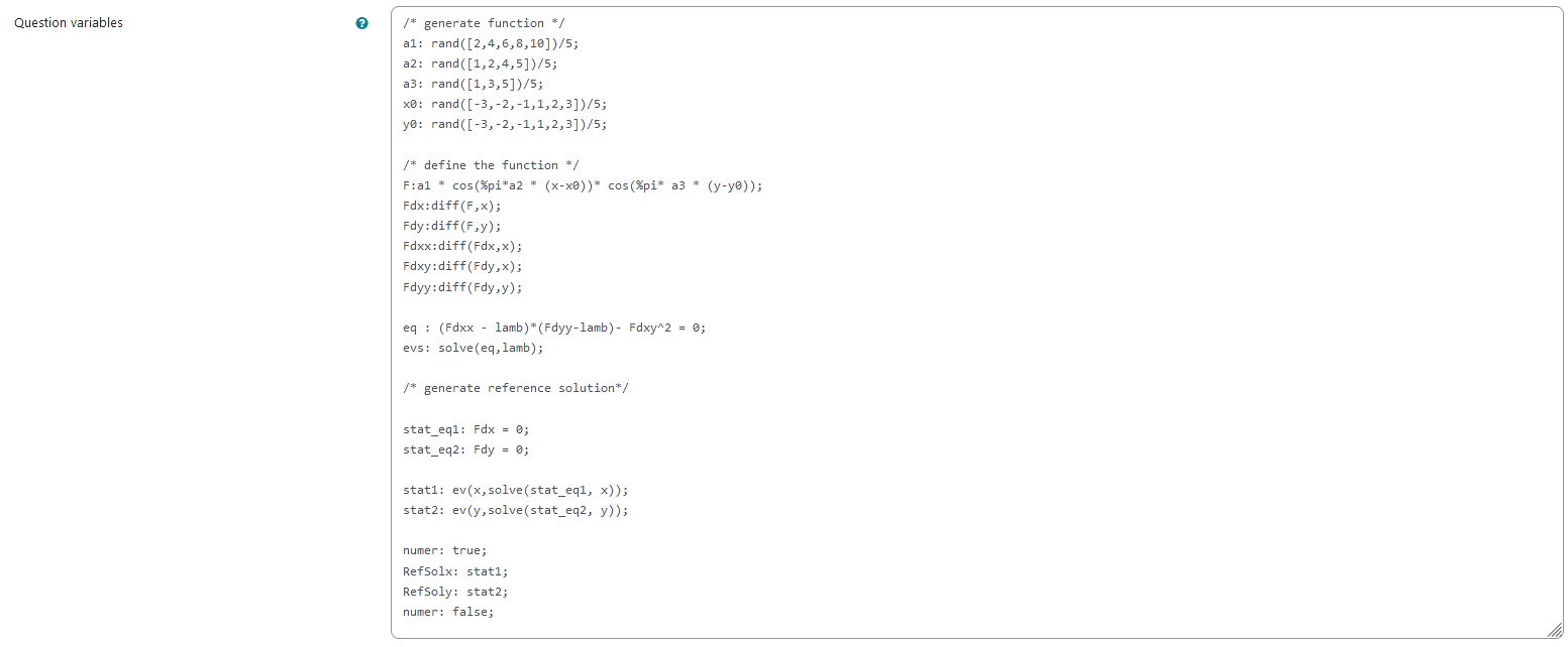
| The above image shows which values the teacher may wish to change |
|
|:–:|
| The above image shows which values the teacher may wish to change |
Question code
Question Variables
- 5 lists of integer numbers for variables
a1,a2,a3,x0andy0to randomly select from - Selected number can be divided or multiplied with a number to scale e.g.:
a1:rand([2,4,6,8,10])/5; -
function F using
a1,a2,a3,x0andy0dependent on variablesx,yas follows:F:a1 * cos(%pi*a2 * (x-x0))* cos( a3 * (y-y0));
Note that this function’s parametersa1,a2,a3,x0andy0are randomized upon executing the code as mentioned above - derivatives of Function F using Maxima syntax e.g.:
Fdx: diff(F,x)to calculate the components of the Hessian Matrix - numerical reference solution e.g.:
RefSolx: stat1;withstat1being the coordinate of a stationary point. `
Question variable code
/* generate function */
a1: rand([2,4,6,8,10])/5;
a2: rand([1,2,4,5])/5;
a3: rand([1,3,5])/5;
x0: rand([-3,-2,-1,1,2,3])/5;
y0: rand([-3,-2,-1,1,2,3])/5;

/* define the function */
F:a1 * cos(%pi*a2 * (x-x0))* cos(%pi* a3 * (y-y0));
Fdx:diff(F,x);
Fdy:diff(F,y);
Fdxx:diff(Fdx,x);
Fdxy:diff(Fdy,x);
Fdyy:diff(Fdy,y);

eq : (Fdxx - lamb)*(Fdyy-lamb)- Fdxy^2 = 0;
evs: solve(eq,lamb);

/* generate reference solution*/

stat_eq1: Fdx = 0;
stat_eq2: Fdy = 0;

stat1: ev(x,solve(stat_eq1, x));
stat2: ev(y,solve(stat_eq2, y));

numer: true;
RefSolx: stat1;
RefSoly: stat2;
numer: false;
Question Text
- “Find a point with a negative-definite Hessian of the function at this point.”
- JSXGraph applet using the functions and variables defined in Question variables plotting the randomized function and displaying the Taylor-Approximation in a point of freely adjustable x,y-coordinates
[[input:ans1]]at the end of JSXGraph code to allow input of an answer of the student[[validation:ans1]]checking of answer
Question text code
<p>Given is the graph of a function and its quadratic approximation around a point. You can move that point by moving its projected point in \(x,y\)-direction. You can rotate the coordinate system using the sliders.</p>
<p>Find a point with a negative-definite Hessian of the function at this point.</p>


[[jsxgraph width="500px" height="500px" input-ref-ans1='ans1Ref']]
var board = JXG.JSXGraph.initBoard(divid,{boundingbox : [-10, 10, 10,-10], axis:false, shownavigation : true});

   var box = [-2, 2];
		    var view = board.create('view3d',
		        [
		            [-6, -3], [8, 8],
		            [box, box, box]
		        ],
		        {
		            xPlaneRear: {visible: false},
		            xPlaneRearYAxis: {visible: false},
		            xPlaneRearZAxis: {visible: false},
		            yPlaneRear: {visible: false},
		            yPlaneRearXAxis: {visible: false},
		            yPlaneRearZAxis: {visible: false},
		        });

                               var txtraw = '{#F#}';
                               txtraw=txtraw.replace(/%pi/g, "PI");
                               //txtraw=txtraw.replace(/pi/g, "PI");
                               var F =  board.jc.snippet(txtraw, true, 'x,y');
                               txtraw = '{#Fdx#}';
                               txtraw=txtraw.replace(/%/g, "");
                               txtraw=txtraw.replace(/pi/g, "PI");
                               var Fdx =  board.jc.snippet(txtraw, true, 'x,y');
                               var txtraw = '{#Fdy#}';
                               txtraw=txtraw.replace(/%/g, "");
                               txtraw=txtraw.replace(/pi/g, "PI");
                               var Fdy =  board.jc.snippet(txtraw, true, 'x,y');
var txtraw = '{#Fdxx#}';
                               txtraw=txtraw.replace(/%/g, "");
                               txtraw=txtraw.replace(/pi/g, "PI");
                               var Fdxx =  board.jc.snippet(txtraw, true, 'x,y');
var txtraw = '{#Fdyy#}';
                               txtraw=txtraw.replace(/%/g, "");
                               txtraw=txtraw.replace(/pi/g, "PI");
                               var Fdyy =  board.jc.snippet(txtraw, true, 'x,y');
var txtraw = '{#Fdxy#}';
                               txtraw=txtraw.replace(/%/g, "");
                               txtraw=txtraw.replace(/pi/g, "PI");
                               var Fdxy =  board.jc.snippet(txtraw, true, 'x,y');
var txtraw = '{#evs[1]#}';
                               txtraw=txtraw.replace(/%/g, "");
                               txtraw=txtraw.replace(/pi/g, "PI");
                               var evs1 =  board.jc.snippet(txtraw, true, 'x,y');
var txtraw = '{#evs[2]#}';
                               txtraw=txtraw.replace(/%/g, "");
                               txtraw=txtraw.replace(/pi/g, "PI");
                               var evs2 =  board.jc.snippet(txtraw, true, 'x,y');

    var c = view.create('functiongraph3d', [
        F,
        box,
        box,
    ], { strokeWidth: 0.5, stepU: 70, stepsV: 70, strokeColor: '#1f84bc'});

  // 3D points:
    // Point on xy plane
    var Axy = view.create('point3d', [1, 1, -2], { withLabel: false });

    // Project Axy to the surface
    var A = view.create('point3d', [
        () => [Axy.X(), Axy.Y(), F(Axy.X(), Axy.Y())]
        ], { withLabel: false, fixed: true});
    view.create('line3d', [Axy, A], { dash: 1 });


   var TF = (x,y) => F(Axy.X(),Axy.Y())+Fdx(Axy.X(),Axy.Y())*(x-Axy.X())
                                         +Fdy(Axy.X(),Axy.Y())*(y-Axy.Y())
                                         +Fdxx(Axy.X(),Axy.Y())*(x-Axy.X())*(x-Axy.X())
                                         +Fdyy(Axy.X(),Axy.Y())*(y-Axy.Y())*(y-Axy.Y())
                                         +2*Fdxy(Axy.X(),Axy.Y())*(y-Axy.Y())*(x-Axy.X());
   var c2 = view.create('functiongraph3d', [
       TF,
       () => [Axy.X()-0.5,Axy.X()+0.5],
       () => [Axy.Y()-0.5,Axy.Y()+0.5,],
   ], { strokeWidth: 0.25, stepU: 50, stepsV: 50, strokeColor: '#EE442F'});


board.update()

var p1 =board.create('point',[function () {return Axy.X();} ,function () {return Axy.Y();}],{visible:false});
stack_jxg.bind_point(ans1Ref,p1);
var stateInput = document.getElementById(ans1Ref);
stateInput.style.display = 'none';


board.update();

 /* axis labels*/
                       var xlabel=view.create('point3d',[0.9*box[1],0,(0.6*box[0]+0.4*box[1])], {size:0,name:"x"});
                       var ylabel=view.create('point3d',[0,0.9*box[1],(0.6*box[0]+0.4*box[1])], {size:0,name:"y"});
                       var zlabel=view.create('point3d',[
                           0.7*(0.6*box[0]+0.4*box[1]),
                           0.7*(0.6*box[0]+0.4*box[1]),
                           0.9*box[1]],
                           {size:0,name:"z"});

[[/jsxgraph]]
<div style="display:none;">
<p>[[input:ans1]] </p><p>[[validation:ans1]]</p></div>
Answers
Answer ans 1
| property | setting |
|---|---|
| Input type | Numerical |
| Model answer | [RefSolx, RefSoly] defined in Question variables |
| Forbidden words | none |
| Forbid float | No |
| Student must verify | Yes |
| Show the validation | Yes, with variable list |
General Feedback
<hr>
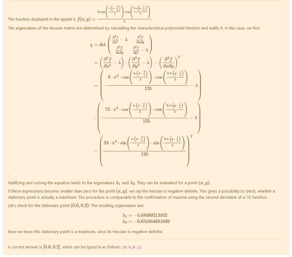
<p> The function displayed in the applet is \(f(x,y) = {@F@} \). </p>
<p> The eigenvalues of the hessian matrix are determined by calculating the characterisitcal polynomial function and nullify it. In this case, we find
\[\begin{align*}
\chi &= \text{det}
\begin{pmatrix}
\frac{\partial ^2 f}{\partial x^2}- \lambda & \frac{\partial ^2 f}{\partial x \partial y} \\
\frac{\partial ^2 f}{\partial x \partial y} & \frac{\partial ^2 f}{\partial y^2}- \lambda
\end{pmatrix}\\
&= \left( \frac{\partial ^2 f}{\partial x^2}- \lambda \right) \cdot \left( \frac{\partial ^2 f}{\partial y^2}- \lambda \right) - \left( \frac{\partial ^2 f}{\partial x \partial y} \right)^2\\
&= \left( {@Fdxx@}- \lambda \right)\\
& \cdot \left( {@Fdyy@}- \lambda \right) \\
&- \left( {@Fdxy@} \right)^2
\end{align*} \] .</p>
<p> Nullifying and solving the equation leads to the eigenvalues \(\lambda_1\) and \(\lambda_2\). They can be evaluated for a point \((x,y)\). </p>
<p> If these expressions become smaller than zero for the point \((x,y)\), we say the hessian is negative-definite. This gives a possibility to check, whether a stationary point is actually a maximum. The procedure is comparable to the confirmation of maxima using the second derivative of a 1D function. </p>
<p> Let's check for the stationary point \(({@ev(x0, numer)@},{@ev(y0, numer)@})\)! The resulting eigenvalues are:
\[\begin{align*}
\lambda_1 &= {@ev(lamb, ev(evs[1], numer, x= x0, y = y0))@} \\
\lambda_2 &= {@ev(lamb, ev(evs[2], numer, x= x0, y = y0))@}
\end{align*} \]
</p>
<p> Now we know this stationary point is a maximum, since its Hessian is negative-definite! </p>
Potential response tree
prt1
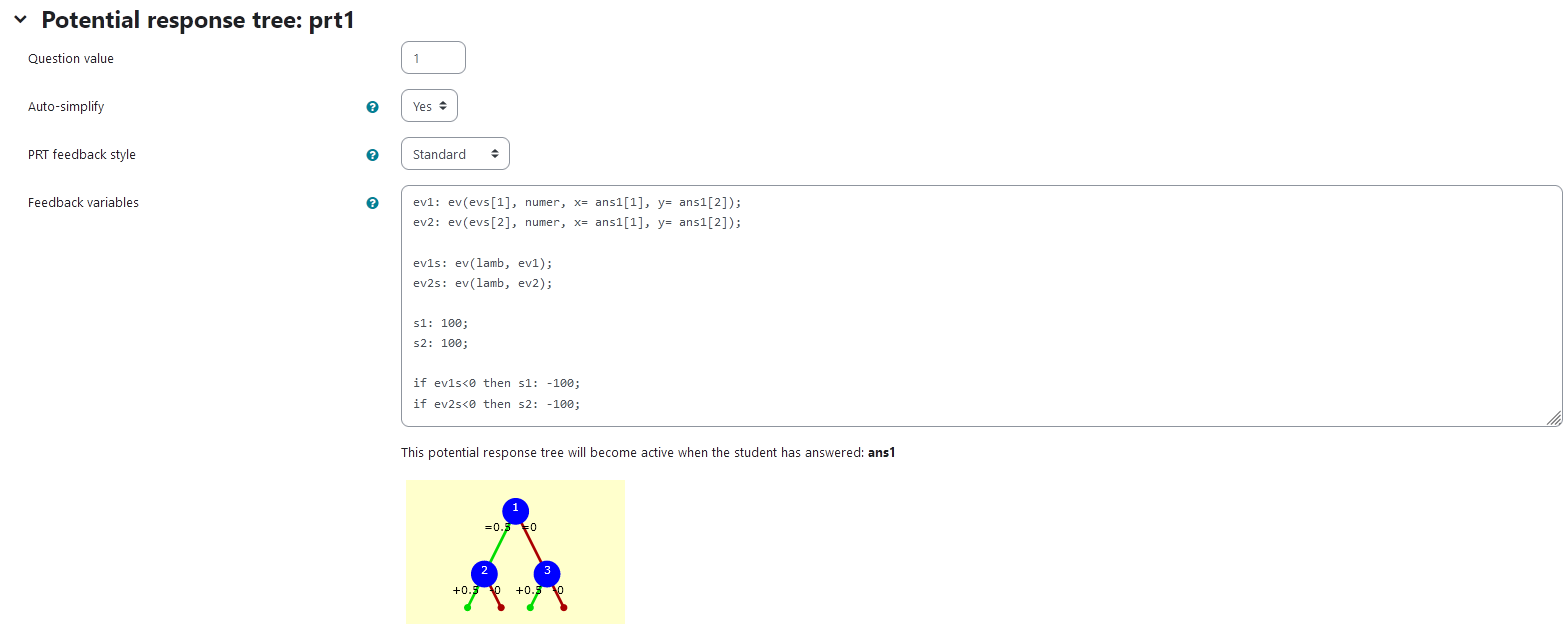
Feedback variables:
ev1: ev(evs[1], numer, x= ans1[1], y= ans1[2]);
ev2: ev(evs[2], numer, x= ans1[1], y= ans1[2]);

ev1s: ev(lamb, ev1);
ev2s: ev(lamb, ev2);

s1: 100;
s2: 100;

if ev1s<0 then s1: -100;
if ev2s<0 then s2: -100;
Creates variables ev1 and ev2by evaluating the formula for the matrix’ eigenvalues at the location selected by the student. Since STACK gives this solution as an equation of type “lamb = {solution}”, it needs to be evaluated once more.
We do so creating the variables ev1sand ev2s. These are the eigenvalues at the selected point.
To be able to check, whether the Hessian is negative-definite or not, we need to check the sign of the eigenvalues. Since STACK expects us to check a numeric answer, we cannot assign the bools trueand false. We create a similar variable instead with s1 and s2 having either of the values 100 or -100.
If the eigenvalues are negative, we assign s1and s2 the value -100.
 |
|---|
| Visualization of PRT 1 |
Node 1
| property | setting |
|---|---|
| Answer Test | NumAbsolute |
| SAns | s1 |
| TAns | -100 |
| Node 1 true feedback | <p>The first eigenvalue is smaller than zero. </p> |
| Node 1 false feedback | <p>The first eigenvalue is not smaller than zero. </p> |
 |
|---|
| Values of node 1 |
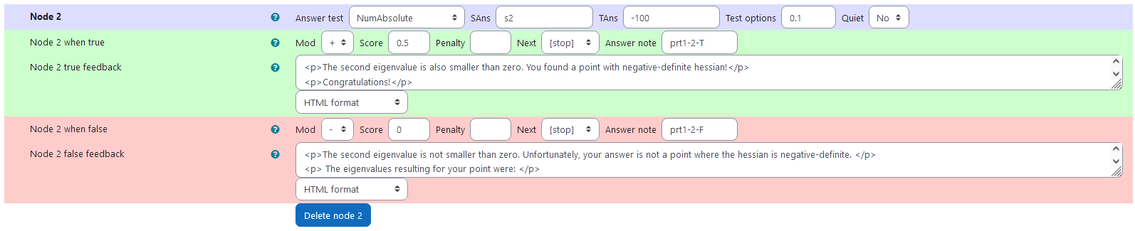
Node 2
| property | setting |
|---|---|
| Answer Test | NumAbsolute |
| SAns | s2 |
| TAns | -100 |
| Node 2 true feedback | <p>The second eigenvalue is also smaller than zero. You found a point with negative-definite hessian!</p><p>Congratulations!</p><p> The eigenvalues resulting for your point were: </p><p> \[\begin{align*}\lambda_1 &= {@ev1s@}\\ \lambda_2 &= {@ev2s@} \end{align*} \] </p> |
| Node 2 false feedback | <p>The second eigenvalue is not smaller than zero. Unfortunately, your answer is not a point where the hessian is negative-definite. </p><p> The eigenvalues resulting for your point were: </p><p> \[\begin{align*} \lambda_1 &= {@ev1s@}\\ \lambda_2 &= {@ev2s@} \end{align*} \] </p> |
 |
|---|
| Values of node 2 |
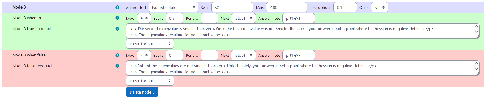
Node 3
| property | setting |
|---|---|
| Answer Test | NumAbsolute |
| SAns | s2 |
| TAns | -100 |
| Node 3 true feedback | <p>The second eigenvalue is smaller than zero. Since the first eigenvalue was not smaller than zero, your answer is not a point where the hessian is negative-definite. </p><p> The eigenvalues resulting for your point were: </p><p> \[\begin{align*} \lambda_1 &= {@ev1s@}\\ \lambda_2 &= {@ev2s@} \end{align*} \] </p> |
| Node 3 false feedback | <p>The second eigenvalue is smaller than zero. Since the first eigenvalue was not smaller than zero, your answer is not a point where the hessian is negative-definite. </p><p> The eigenvalues resulting for your point were: </p><p> \[\begin{align*} \lambda_1 &= {@ev1s@}\\\lambda_2 &= {@ev2s@} \end{align*} \] </p> |
 |
|---|
| Values of node 3 |